Last week (1st- 4th of July) I attended the Senior Physics Challenge boot camp held at Churchill college, Cambridge. 41 attendees were selected due to high performance in the Senior Physics Challenge (which ran from the end of last year to April this year) in which students answer questions of varying difficulty across different areas of physics including mechanics, waves, fields and circuits. The Senior Physics Challenge (SPC) bootcamp looked at an introduction to quantum mechanics. Throughout the week we had lectures in the Pippard lecture theatre held by Professor Mark Warner and solved problems from the Cavendish Quantum Mechanics Primer (co-written by Professor Warner).
…………………………………………………………………………………………………………………….
Topic covered during the week included the wave functions of particles ψ(x), Schrodinger’s Equation, quantisation, confinement energy, localisation, as well as infinite and finite square well potentials. Before arriving we had individually worked through chapter one which covered the movement from classical to quantum (the movement to potentials rather than forces and how forces are the negative derivative of potentials) and mathematical preliminaries.
Wave functions of particles and the Heisenberg uncertainty principle
Partially covered in Chapter One of the primer, particles can be represented using a wave function, ψ(x), where the x-axis is the position of the particle and the where probability of finding the particles at the position x (the probability density P(x)) is equal to the wavefunction squared, |ψ(x)|^2.
This leads on into the Heisenberg uncertainty principle which states:
Δ x. Δ p ⩾ 1/2 ħ
where ħ (“h bar”- it might have a technical name but I don’t know it) is plank’s constant, h, over 2 pi –> h/(2π)
Simply put, the uncertainty in x (i.e. how uncertain we are about where the particle is) multiplied by the uncertainty in momentum, p, is equal to or greater than a constant, ħ. Therefore, the more we know about the position of a particle, the less sure we are of its momentum and vice versa. Also useful to keep in mind is using the momentum to find out (roughly) kinetic energy. While previously, I had always known KE = 1/2mv^2, in quantum mechanics KE (often represented as T) is momentum (p) squared, divided by 2m. Thinking about kinetic energy in terms of momentum is more useful when it comes to quantum mechanics it turns out because of momentum being used in other equations ( such as the Heisenberg uncertainty principle).
Schrodinger’s Equation
Schrodinger’s equation is a differential equations which describes the wavefunction of a quantum-mechanical system. It was and still is extremely significant in the world of quantum mechanics.
In quantum mechanics, measurable quantities become operators. Operators are denoted by a little hat (^) about the character. For example kinetic energy T(x) becomes T-hat, and potential energy V(x) becomes V-hat.
Eigenvalues and Eigenfunctions
Best demonstrated using an example:

The H-hat (called the Hamiltonian operator- it’s important later) acts on the wave function, ψ(x). The result is a value, E multiplied y the original function, ψ(x). When an operator acts on a function and produces the original function, the function is called an eigenfunction and the value multiplied by the function (in this case E) is called the eigenvalue.
Returning to the Hamiltonian, it is comprised of two operators, T-hat, the kinetic energy operator, and V-hat, the potential energy operator:


The Hamiltonian links to the total energy, which is the kinetic energy plus the potential energy. Subbing in the value of T-hat into Equation 1, we get what is called the time-independent Schrodinger equation:

The reason it’s so specifically called the time-independent Schrodinger Ewuation is because there’s actually a time-dependant Schrodinger Equation.
Now, we’ve looked at the basics of Schrodinger’s equation, there are some postulates of quantum mechanics which are useful to look at, remember and most importantly, understand.
- The state of a quantum mechanical system depends on the function ψ(x, t) where x is position of the particle and t is time.
- |ψ(x)|^2 dx is the probability the particle is between x and x + dx.
- For every measurable quantity in classical mechanics (for example T) there is an operator in quantum mechanics (T-hat)
There’s a couple more but those are good enough for now.
The infinite square well potential

In a one-dimensional infinite square well potential there is a particle in a box. Picture the box as two lines a distance L apart. The particle (for now) can only move in the box, it cannot go through the walls- it is confined to the box. In the well the potential of the particle is zero.

Looking at the first two states, there is the ground state and the first excited state of the particle shown by two wavefunctions. Looking to the left, A is the particle confined within the well. B is the ground state- it has one antinode and no nodes (the nodes at the edges aren’t counted). C is the first excited state- it has two antinodes and one node. D is the second excited state and so on, the pattern continues. The confinement of a particle within a well is called localisation (the process of “localising” a particle).
Inside the well (as the potential energy of the particle is zero) Schrodinger’s equation becomes:
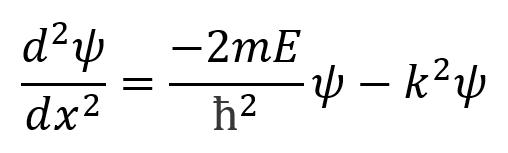
where k = (2mE)^1/2/ ħ (the square root of 2mE divided by h-bar)
This equations had solutions of ψ proportional to sin(kx) and ψ proportional to cos(kx). By looking at the boundary conditions: ψ must be 0 at x = 0 (we can see this on the graph) that at the start of the well the wavefunctions both have value 0. Plugging x = 0 into solutions sin(kx) and cos(kx) we see that only sin(kx) is equal to 0 (cos(0) = 1). So we have refined our solutions to be just sin(kx). Looking at the other boundary condition, at L the wavefunctions are also equal to 0. Therefore, kx must be equal to nπ where n is any positive integer (1,2,3… because sin(π), sin(2π), sin(3π) etc are all equal to 0). So sin(kx) is a solution.
Energy
Looking back at the Heisenberg uncertainty principle, Δ x. Δ p ⩾ 1/2 ħ . By confining a particle we reduce the uncertainty of its position, thus increasing the uncertainty of the particle’s momentum. If T = p^2/2m and from the Heisenberg uncertainty principle, p = ħ/Δ x (roughly)- we can say T = ħ ^2/(2m( Δ x )^2) (by confining the two equations). This is the confinement energy and is caused, unsurprisingly, from the confinement of the particle. More specifically, it comes from the momentum that localisation (mentioned above) creates. T can also be shown to be equal to:

Where n is the state (ground state n = 1 and so on). This is also equal to the energy of the ground state, E1, multiplied by n^2.
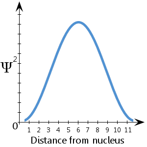
One other thing we looked at was the probability distributions of the particle in some of its various states, ground state (n = 1) and the first excited state (n = 2). As mentioned before, P(x) is proportional to |ψ(x)|^2, so the probability distributions ended up looking at little like this:

Sturm-Liouville Theory

The part of the Sturm-Liouville theory shows that the curvature of the wavefunction is proportional to the kinetic energy (as E = V + T, then T = E – V). If there is a greater curvature the wavefunction bends quicker so reaches the next node faster. Therefore, in the same distance L, the higher the kinetic energy of the state the more nodes the state will have. This is why the ground state has 0 nodes, the first excited state has 1 node, the second excited state has 2 nodes and so on.
Heisenberg and Coulomb
Looking at electrons in atoms required combining the Heisenberg uncertainty principle and the Coulomb potential energy, V(x) = Q1Q2/(4πεx) where ε (eplison symbol) is the permittivity of free space, Q1 and Q2 are are the charges of two particles, and x is the distance between the two particles.
Now, consider if the nucleus of an atom has a charge of Ze, the energy of an electron is the electric field of a nucleus is -Ze^2/(4πεr). The energy is negative because the two charges are opposite (one positively charged, the other negatively charged). Localisation of the electron means there will be quantum kinetic energy, ħ^2 / (2mr^2) as well.
Overall, the total electronic energy is the sum of the confinement kinetic energy ( ħ^2 / (2mr^2) ) plus the electrical attraction to the proton (which is negative):
E = ħ^2 / (2mr^2) – Ze^2/(4πεr)
The first derivative of E (dE/dr) and setting it to zero gives the Bohr radius- the “size” of a hydrogen atom (in this case).
There’s a couple more things we covered like a quick introduction of relativity and quantum mechanics, finite square wells and harmonic potential wells but they’re all topics I would like to go over a couple more times before writing about!
Thank you for reading! If you enjoyed this, you might like:
- Norimaki Synthesizer Taste Display: a tasty sample of science
- Applying to Cambridge Natural Sciences, a guide
- Michael Crichton, an author to remember
- Taking Lego down to near absolute zero with the first Lego cryonaut
- The standardisation of espresso flavour using maths
References

I was suggested this website by my cousin. I am not sure whether this post is
written by him as no one else know such detailed about my trouble.
You’re incredible! Thanks!
LikeLike